Introduction
Although they can be run individually for specific analysis cases, these codes are often run in combination. Whilst 3D numerical simulation is becoming more common-place, 2D analysis still has its place. As long as they are applied correctly (requiring the user to have a good understanding of their limitations), 2D methods can offer an efficient means to simulate the icing problem. With each simulation taking a few tens of seconds (up to a few minutes for multi-step cases), hundreds of calculations can easily be performed without High Performance Computing capability. Lifting surface analysis (wings, empennage, rotors and propellers) can all successfully be performed in 2D.
The TAC2 code can be used to calculate the trajectories of cloud water droplets and resultant water droplet catch efficiency distribution on a multi-element 2D body in incompressible flow. It can be used to establish the amount and location of water droplet impact on a body, which is a pre-curser to the calculation of ice accretion shape and size, and in the modelling of ice protection systems.

The IHB code performs a steady-state ‘Messinger’ type heat balance on the outer surface of the geometry, to calculate the local freezing fraction and surface temperature. This allows the ice growth rate to be determined, and hence the ice shape for a given encounter time.
External heat can also be specified in IHB at various chord-wise locations to simulate the heat input from an ice protection system, and the code will calculate whether ice still grows, the surface runs wet, or the water is fully evaporated. In this way, the IHB code provides a simple method to gain data on the potential power needs for an anti-ice system, early in the design process.
Technical
The TAC2 code uses a Lagrangian particle tracking technique to calculate the trajectory of a cloud water droplet from a starting position upstream of the aerofoil under investigation. The position of the droplet is integrated in small steps until either the droplet impacts the aerofoil or it passes defined boundaries (used to signify a ‘miss’ trajectory). A fourth order Runge-Kutta technique is used to integrate the equations of motion, which assume only aerodynamic drag and gravity affects the droplet motion. The integration requires the local velocity components to be known at every position the droplet occupies. In the TAC code, the required velocity data are calculated using a 2D, multi-element, incompressible flow, panel method which is based on linear varying vorticity on each panel. The code calculates the limiting trajectory (i.e. tangential to the aerofoil surface) on each of the upper and lower surfaces on a user specified number of the aerofoil components. Once the limit trajectories are found the code automatically launches ‘intermediate’ trajectories to get the detailed impingement locations. A cubic spline fit is made to the initial point (‘Y0’) and impact point (‘s/c’), with a zero gradient end slope condition applied at the limiting trajectory points. The slope of the cubic spline is then evaluated at a series of points about the aerofoil leading edge, which corresponds to the local water droplet catch efficiency, β. The code also calculates the ‘overall’ catch efficiency, E, which is expressed as the separation between the two limiting trajectories in the free stream relative to the projected height of the aerofoil. Finally, using the panel method calculated surface velocity data, the code conducts an integral boundary layer calculation for a rough surface to predict the local surface convective heat transfer coefficient distribution, which is output, along with pressure coefficient and catch distribution, in the format required by simulation tools IHB and ET3D.
TAC2 can automatically calculate the catch efficiency for a spectrum of droplet sizes (e.g. for a Langmuir-D distribution, or th Standard 10-bin Freezing Rain distribution (for median volumetric diameters either less than or greater than 40 microns). The code also includes ‘splash’ and ‘bounce’ models which are used for larger droplet conditions such as Freezing Drizzle and Freezing Rain. These account for the specific effects of larger droplets which are known to occur, and reduce the surface water collection efficiency.
TAC2 and IHB can perform multi-step calculations, allowing the effect of the ice shape on the velocity and impingement profiles to be re-assessed at reguar intervals. Large ice shapes can have a significant effect on the flow, and this mult-step process allows more accurate prediction of such shapes.
Whilst the standard mode of running IHB is to produce an ice shape without any form of active protection, the code does also allow initial assessment of the power demand for an anti-ice system. Only steady-state performance is considered, because the structure itself is not modelled. One mode allows the ‘ideal’ power to be determined. This is the power input needed to maintain the surface at 0°C, and is therefore the minimum value which would be needed from an anti-ice system. It is named ‘ideal’ because, in practice, tolerances must be accounted for. Therefore, the code also allows the user to specify a desired surface temperature (e.g. +5°C), allowing a more representative power demand to be calculated. Both of these options allow the power input to vary at each calculation node around the surface, which is not realistic for an actual system. A final run type option therefore exists where the user can specify fixed power inputs over different regions of the surface and determine whether ice forms, the surface is kept in a running-wet state (temperature above 0°C), or is fully-evaporative. This assessment is generally a pre-cursor to a more detailed analysis using the ET3D simulation tool.
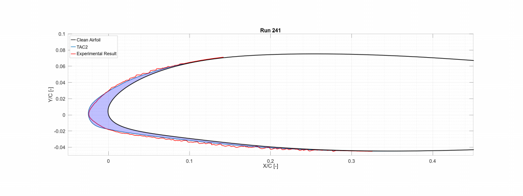
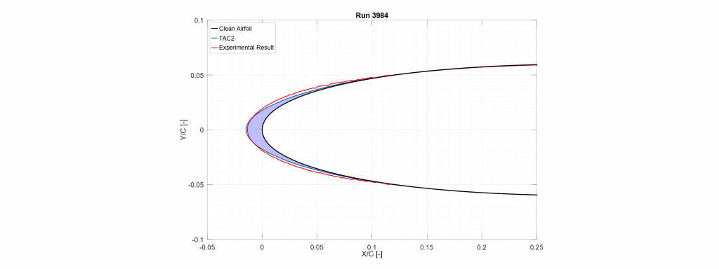
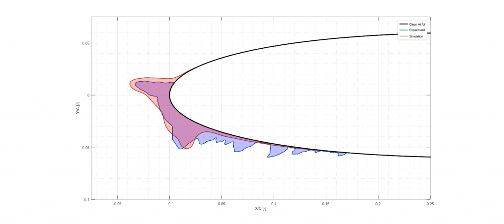
Example Comparisons
A wide range of experimental data is available to compare the 2D simulatio tools against. A few examples are shown below.